Finding Profitable Entry Points with NumPy: A Data-Driven Strategy to Beat the Market
Every investor dreams of beating the market. While timing the market perfectly is impossible, what if we could identify specific entry points—percentage drops from recent highs—that historically offer high probabilities of outperformance? If we can't, let's just invest in indexes.
Software Engineer
Schild Technologies

Finding Profitable Entry Points with NumPy: A Data-Driven Strategy to Beat the Market
Every investor dreams of beating the market. While timing the market perfectly is impossible, what if we could identify specific entry points—percentage drops from recent highs—that historically offer high probabilities of outperformance? If we can't, let's just invest in indexes. Using Python and NumPy, we can analyze years of stock price data to find these optimal entry thresholds.
In this article, we'll use NumPy to analyze ten years of daily closing prices for a stock, identify various entry strategies based on percentage drops, and compare their long-term performance against market benchmarks like the S&P 500.
The core question
When a stock drops from its recent high, at what percentage drop does buying become statistically advantageous for long-term holders? Should you buy after a 5% dip? 10%? 20%? And over what holding periods does this strategy work best?
Why NumPy for financial analysis?
NumPy excels at financial time series analysis for several reasons:
- Vectorized operations: Calculate percentage changes across thousands of days instantly
- Efficient memory usage: Handle decade-long daily price data without performance issues
- Statistical functions: Built-in tools for means, standard deviations, and percentiles
- Array slicing: Easily analyze specific time windows and holding periods
Let's get started.
Setting up our analysis
First, let's import our dependencies and get our market data. We'll be using real JPM and VOO (S&P 500 ETF) data from Yahoo Finance. JPM is JPMorgan Chase & Co., and VOO is a Vanguard index.
import numpy as np
import matplotlib.pyplot as plt
from datetime import datetime, timedelta
import yfinance as yf

# Download real JPM stock data
stock_data = yf.download('JPM', start='2015-01-01', end='2025-01-01')
stock_prices = stock_data['Close'].values

# Download real VOO (S&P 500 ETF) data
voo_data = yf.download('VOO', start='2015-01-01', end='2025-01-01')
sp500_prices = voo_data['Close'].values

# Make sure they have matching dates (remove any gaps)
common_dates = stock_data.index.intersection(voo_data.index)
stock_prices = stock_data.loc[common_dates, 'Close'].values
sp500_prices = voo_data.loc[common_dates, 'Close'].values
dates = common_dates.values
n_days = len(stock_prices)

# Calculate actual total returns
jpm_total_return = ((stock_prices[-1] / stock_prices[0]) - 1) * 100
voo_total_return = ((sp500_prices[-1] / sp500_prices[0]) - 1) * 100

print(f"JPM price range: ${stock_prices.min():.2f} to ${stock_prices.max():.2f}")
print(f"VOO (S&P 500) range: ${sp500_prices.min():.2f} to ${sp500_prices.max():.2f}")
print(f"Number of trading days: {n_days}")
print(f"JPM actual total return: {float(jpm_total_return):.1f}%")
print(f"VOO actual total return: {float(voo_total_return):.1f}%")

# JPM price range: $40.66 to $245.10
# VOO (S&P 500) range: $141.95 to $551.83
# Number of trading days: 2516
# JPM actual total return: 402.4%
# VOO actual total return: 241.8%
Calculating rolling maximum and drawdowns
To identify "buying opportunities," we need to know how far a stock has dropped from its recent peak. We'll calculate rolling maximums and current drawdowns:
def calculate_drawdowns(prices, window=252):
    """
    Calculate percentage drawdown from rolling maximum.

    Args:
        prices: Array of daily closing prices
        window: Lookback period in days (252 = 1 year of trading days)

    Returns:
        Array of drawdown percentages (negative values)
    """
    # Calculate rolling maximum using a sliding window
    rolling_max = np.zeros_like(prices)

    for i in range(len(prices)):
        start_idx = max(0, i - window + 1)
        rolling_max[i] = np.max(prices[start_idx:i+1])

    # Calculate drawdown percentage
    drawdowns = ((prices - rolling_max) / rolling_max) * 100

    return drawdowns, rolling_max

# Calculate 1-year rolling maximum and drawdowns
drawdowns, rolling_max = calculate_drawdowns(stock_prices, window=252)

print(f"Maximum drawdown: {drawdowns.min():.2f}%")
print(f"Average drawdown: {drawdowns.mean():.2f}%")
print(f"Days with >10% drawdown: {np.sum(drawdowns < -10)}")

# Maximum drawdown: -43.63%
# Average drawdown: -8.42%
# Days with >10% drawdown: 696
Identifying entry points
Now we'll identify specific days when the stock dropped below certain thresholds from its recent high:
def identify_entry_points(prices, drawdowns, thresholds):
    """
    Identify days when price drops below specified thresholds.

    Args:
        prices: Array of daily prices
        drawdowns: Array of drawdown percentages
        thresholds: List of drawdown thresholds (e.g., [-5, -10, -15, -20])

    Returns:
        Dictionary mapping thresholds to arrays of entry point indices
    """
    entry_points = {}

    for threshold in thresholds:
        entries = []
        in_drawdown = False

        for i in range(len(drawdowns)):
            # Check if we just entered a drawdown below threshold
            if drawdowns[i] < threshold and not in_drawdown:
                entries.append(i)
                in_drawdown = True
            # Check if we recovered above threshold
            elif drawdowns[i] >= threshold and in_drawdown:
                in_drawdown = False

        entry_points[threshold] = np.array(entries)

    return entry_points

# Define our test thresholds
thresholds = [-5, -10, -15, -20, -25, -30]
entry_points = identify_entry_points(stock_prices, drawdowns, thresholds)

# Display entry point statistics
for threshold, entries in entry_points.items():
    print(f"\nThreshold {threshold}%:")
    print(f"  Number of entry opportunities: {len(entries)}")
    print(f"  Average days between entries: {np.diff(entries).mean():.1f}" if len(entries) > 1 else "  N/A")

# Threshold -5%:
#   Number of entry opportunities: 68
#   Average days between entries: 37.4
#
# Threshold -10%:
#   Number of entry opportunities: 37
#   Average days between entries: 66.8
#
# Threshold -15%:
#   Number of entry opportunities: 16
#   Average days between entries: 102.8
#
# Threshold -20%:
#   Number of entry opportunities: 12
#   Average days between entries: 158.5
#
# Threshold -25%:
#   Number of entry opportunities: 10
#   Average days between entries: 63.2
#
# Threshold -30%:
#   Number of entry opportunities: 20
#   Average days between entries: 34.7
Calculating returns for different holding periods
The critical question: Do these entry points actually lead to outperformance? Let's calculate returns for various holding periods:
def calculate_forward_returns(prices, entry_indices, holding_periods):
    """
    Calculate returns from entry points over various holding periods.

    Args:
        prices: Array of daily prices
        entry_indices: Array of entry point indices
        holding_periods: List of holding periods in days (e.g., [252, 756, 1260])

    Returns:
        Dictionary mapping holding periods to arrays of returns
    """
    returns_by_period = {}

    for period in holding_periods:
        returns = []

        for entry_idx in entry_indices:
            # Ensure we have enough data after entry
            if entry_idx + period < len(prices):
                entry_price = prices[entry_idx]
                exit_price = prices[entry_idx + period]

                # Calculate percentage return
                ret = ((exit_price - entry_price) / entry_price) * 100
                returns.append(ret)

        returns_by_period[period] = np.array(returns)

    return returns_by_period

# Define holding periods (in trading days)
# 252 days ≈ 1 year, 756 ≈ 3 years, 1260 ≈ 5 years
holding_periods = [252, 756, 1260]

# Calculate returns for each threshold and holding period
results = {}

for threshold, entries in entry_points.items():
    results[threshold] = calculate_forward_returns(
        stock_prices,
        entries,
        holding_periods
    )

# Display results
print("\n=== Returns by Entry Threshold and Holding Period ===\n")

for threshold in thresholds:
    print(f"Entry Threshold: {threshold}%")

    for period in holding_periods:
        years = period / 252
        returns = results[threshold][period]

        if len(returns) > 0:
            print(f"  {years:.0f}-year holding period:")
            print(f"    Mean return: {returns.mean():.2f}%")
            print(f"    Median return: {np.median(returns):.2f}%")
            print(f"    Win rate: {(returns > 0).sum() / len(returns) * 100:.1f}%")
            print(f"    Number of trades: {len(returns)}")
        else:
            print(f"  {years:.0f}-year holding period: Insufficient data")

    print()

# === Returns by Entry Threshold and Holding Period ===
#
# Entry Threshold: -5%
#   1-year holding period:
#     Mean return: 8.97%
#     Median return: 2.67%
#     Win rate: 58.1%
#     Number of trades: 62
#   3-year holding period:
#     Mean return: 48.98%
#     Median return: 50.05%
#     Win rate: 98.1%
#     Number of trades: 53
#   5-year holding period:
#     Mean return: 101.44%
#     Median return: 107.07%
#     Win rate: 100.0%
#     Number of trades: 39
#
# Entry Threshold: -10%
#   1-year holding period:
#     Mean return: 23.28%
#     Median return: 24.13%
#     Win rate: 80.6%
#     Number of trades: 36
#   3-year holding period:
#     Mean return: 72.88%
#     Median return: 69.64%
#     Win rate: 100.0%
#     Number of trades: 26
#   5-year holding period:
#     Mean return: 122.02%
#     Median return: 104.17%
#     Win rate: 100.0%
#     Number of trades: 20
#
# Entry Threshold: -15%
#   1-year holding period:
#     Mean return: 36.43%
#     Median return: 44.47%
#     Win rate: 87.5%
#     Number of trades: 16
#   3-year holding period:
#     Mean return: 69.59%
#     Median return: 77.49%
#     Win rate: 100.0%
#     Number of trades: 13
#   5-year holding period:
#     Mean return: 175.89%
#     Median return: 189.20%
#     Win rate: 100.0%
#     Number of trades: 8
#
# Entry Threshold: -20%
#   1-year holding period:
#     Mean return: 32.37%
#     Median return: 32.15%
#     Win rate: 91.7%
#     Number of trades: 12
#   3-year holding period:
#     Mean return: 74.34%
#     Median return: 82.29%
#     Win rate: 100.0%
#     Number of trades: 5
#   5-year holding period:
#     Mean return: 164.50%
#     Median return: 178.87%
#     Win rate: 100.0%
#     Number of trades: 3
#
# Entry Threshold: -25%
#   1-year holding period:
#     Mean return: 51.73%
#     Median return: 63.45%
#     Win rate: 100.0%
#     Number of trades: 10
#   3-year holding period:
#     Mean return: 56.09%
#     Median return: 57.74%
#     Win rate: 100.0%
#     Number of trades: 7
#   5-year holding period: Insufficient data
#
# Entry Threshold: -30%
#   1-year holding period:
#     Mean return: 47.10%
#     Median return: 47.05%
#     Win rate: 100.0%
#     Number of trades: 20
#   3-year holding period:
#     Mean return: 61.44%
#     Median return: 59.92%
#     Win rate: 100.0%
#     Number of trades: 10
#   5-year holding period: Insufficient data
Comparing against the market benchmark
The real test: Do these entry strategies beat a simple buy-and-hold of the S&P 500?
def calculate_benchmark_returns(benchmark_prices, entry_indices, holding_periods):
    """
    Calculate benchmark returns over the same periods.
    """
    benchmark_returns = {}

    for period in holding_periods:
        returns = []

        for entry_idx in entry_indices:
            if entry_idx + period < len(benchmark_prices):
                entry_price = benchmark_prices[entry_idx]
                exit_price = benchmark_prices[entry_idx + period]

                ret = ((exit_price - entry_price) / entry_price) * 100
                returns.append(ret)

        benchmark_returns[period] = np.array(returns)

    return benchmark_returns

# Calculate alpha (excess return over benchmark) for each strategy
print("\n=== Alpha Analysis: Strategy vs S&P 500 ===\n")

for threshold, entries in entry_points.items():
    print(f"Entry Threshold: {threshold}%")

    # Get benchmark returns for same entry points
    benchmark_returns = calculate_benchmark_returns(
        sp500_prices,
        entries,
        holding_periods
    )

    for period in holding_periods:
        years = period / 252
        strategy_returns = results[threshold][period]
        bench_returns = benchmark_returns[period]

        if len(strategy_returns) > 0 and len(bench_returns) > 0:
            # Calculate alpha (average excess return)
            alpha = strategy_returns.mean() - bench_returns.mean()

            # Calculate probability of beating benchmark
            beat_market = strategy_returns > bench_returns
            prob_beat = beat_market.sum() / len(beat_market) * 100

            print(f"  {years:.0f}-year holding period:")
            print(f"    Average alpha: {alpha:.2f}%")
            print(f"    Probability of beating S&P 500: {prob_beat:.1f}%")
            print(f"    Strategy mean: {strategy_returns.mean():.2f}%")
            print(f"    S&P 500 mean: {bench_returns.mean():.2f}%")

    print()

# === Alpha Analysis: Strategy vs S&P 500 ===
#
# Entry Threshold: -5%
#   1-year holding period:
#     Average alpha: -0.97%
#     Probability of beating S&P 500: 45.2%
#     Strategy mean: 8.97%
#     S&P 500 mean: 9.94%
#   3-year holding period:
#     Average alpha: 6.14%
#     Probability of beating S&P 500: 49.1%
#     Strategy mean: 48.98%
#     S&P 500 mean: 42.84%
#   5-year holding period:
#     Average alpha: 9.72%
#     Probability of beating S&P 500: 59.0%
#     Strategy mean: 101.44%
#     S&P 500 mean: 91.72%
#
# Entry Threshold: -10%
#   1-year holding period:
#     Average alpha: 9.05%
#     Probability of beating S&P 500: 69.4%
#     Strategy mean: 23.28%
#     S&P 500 mean: 14.22%
#   3-year holding period:
#     Average alpha: 20.10%
#     Probability of beating S&P 500: 69.2%
#     Strategy mean: 72.88%
#     S&P 500 mean: 52.78%
#   5-year holding period:
#     Average alpha: 24.05%
#     Probability of beating S&P 500: 55.0%
#     Strategy mean: 122.02%
#     S&P 500 mean: 97.98%
#
# Entry Threshold: -15%
#   1-year holding period:
#     Average alpha: 18.43%
#     Probability of beating S&P 500: 100.0%
#     Strategy mean: 36.43%
#     S&P 500 mean: 18.00%
#   3-year holding period:
#     Average alpha: 19.28%
#     Probability of beating S&P 500: 61.5%
#     Strategy mean: 69.59%
#     S&P 500 mean: 50.30%
#   5-year holding period:
#     Average alpha: 57.03%
#     Probability of beating S&P 500: 87.5%
#     Strategy mean: 175.89%
#     S&P 500 mean: 118.86%
#
# Entry Threshold: -20%
#   1-year holding period:
#     Average alpha: 14.00%
#     Probability of beating S&P 500: 91.7%
#     Strategy mean: 32.37%
#     S&P 500 mean: 18.37%
#   3-year holding period:
#     Average alpha: 15.10%
#     Probability of beating S&P 500: 40.0%
#     Strategy mean: 74.34%
#     S&P 500 mean: 59.24%
#   5-year holding period:
#     Average alpha: 38.05%
#     Probability of beating S&P 500: 66.7%
#     Strategy mean: 164.50%
#     S&P 500 mean: 126.44%
#
# Entry Threshold: -25%
#   1-year holding period:
#     Average alpha: 25.49%
#     Probability of beating S&P 500: 100.0%
#     Strategy mean: 51.73%
#     S&P 500 mean: 26.24%
#   3-year holding period:
#     Average alpha: 17.34%
#     Probability of beating S&P 500: 100.0%
#     Strategy mean: 56.09%
#     S&P 500 mean: 38.75%
#
# Entry Threshold: -30%
#   1-year holding period:
#     Average alpha: 18.41%
#     Probability of beating S&P 500: 100.0%
#     Strategy mean: 47.10%
#     S&P 500 mean: 28.70%
#   3-year holding period:
#     Average alpha: 11.25%
#     Probability of beating S&P 500: 90.0%
#     Strategy mean: 61.44%
#     S&P 500 mean: 50.19%
Statistical significance testing
Are our results statistically significant or just luck? Let's use NumPy to perform a basic t-test:
def calculate_ttest(strategy_returns, benchmark_returns):
    """
    Perform paired t-test to determine statistical significance.
    """
    if len(strategy_returns) != len(benchmark_returns) or len(strategy_returns) == 0:
        return None, None

    # Calculate differences
    differences = strategy_returns - benchmark_returns

    # Calculate t-statistic
    mean_diff = np.mean(differences)
    std_diff = np.std(differences, ddof=1)
    n = len(differences)

    if std_diff == 0:
        return None, None

    t_stat = mean_diff / (std_diff / np.sqrt(n))

    # Degrees of freedom
    df = n - 1

    return t_stat, df

print("\n=== Statistical Significance (t-test) ===\n")

for threshold, entries in entry_points.items():
    print(f"Entry Threshold: {threshold}%")

    benchmark_returns = calculate_benchmark_returns(
        sp500_prices,
        entries,
        holding_periods
    )

    for period in holding_periods:
        years = period / 252
        strategy_returns = results[threshold][period]
        bench_returns = benchmark_returns[period]

        t_stat, df = calculate_ttest(strategy_returns, bench_returns)

        if t_stat is not None:
            # Rule of thumb: |t| > 2 suggests significance at 95% confidence
            significant = abs(t_stat) > 2

            print(f"  {years:.0f}-year holding: t-stat = {t_stat:.3f}, df = {df}")
            print(f"    {'*** SIGNIFICANT' if significant else 'Not significant'}")

    print()

# === Statistical Significance (t-test) ===
#
# Entry Threshold: -5%
#   1-year holding: t-stat = -0.497, df = 61
#     Not significant
#   3-year holding: t-stat = 1.564, df = 52
#     Not significant
#   5-year holding: t-stat = 1.600, df = 38
#     Not significant
#
# Entry Threshold: -10%
#   1-year holding: t-stat = 3.907, df = 35
#     *** SIGNIFICANT
#   3-year holding: t-stat = 3.550, df = 25
#     *** SIGNIFICANT
#   5-year holding: t-stat = 2.586, df = 19
#     *** SIGNIFICANT
#
# Entry Threshold: -15%
#   1-year holding: t-stat = 5.370, df = 15
#     *** SIGNIFICANT
#   3-year holding: t-stat = 2.592, df = 12
#     *** SIGNIFICANT
#   5-year holding: t-stat = 4.967, df = 7
#     *** SIGNIFICANT
#
# Entry Threshold: -20%
#   1-year holding: t-stat = 4.170, df = 11
#     *** SIGNIFICANT
#   3-year holding: t-stat = 1.021, df = 4
#     Not significant
#   5-year holding: t-stat = 1.648, df = 2
#     Not significant
#
# Entry Threshold: -25%
#   1-year holding: t-stat = 8.207, df = 9
#     *** SIGNIFICANT
#   3-year holding: t-stat = 5.001, df = 6
#     *** SIGNIFICANT
#
# Entry Threshold: -30%
#   1-year holding: t-stat = 12.667, df = 19
#     *** SIGNIFICANT
#   3-year holding: t-stat = 2.684, df = 9
#     *** SIGNIFICANT
Finding the optimal entry strategy
Now let's synthesize our findings to identify which entry thresholds work best:
def find_optimal_strategy(results, benchmark_returns_all, holding_periods):
    """
    Identify optimal entry strategy based on alpha and win rate.
    """
    best_strategies = {}

    for period in holding_periods:
        years = period / 252
        best_alpha = -np.inf
        best_threshold = None
        best_metrics = None

        for threshold in thresholds:
            strategy_returns = results[threshold][period]

            if threshold not in entry_points:
                continue

            entries = entry_points[threshold]
            benchmark_returns = calculate_benchmark_returns(
                sp500_prices,
                entries,
                holding_periods
            )[period]

            if len(strategy_returns) > 5 and len(benchmark_returns) > 5:  # Minimum sample
                alpha = strategy_returns.mean() - benchmark_returns.mean()
                prob_beat = (strategy_returns > benchmark_returns).sum() / len(strategy_returns) * 100

                # Composite score: alpha + win rate bonus
                score = alpha + (prob_beat - 50) * 0.1  # Small bonus for high win rate

                if score > best_alpha:
                    best_alpha = score
                    best_threshold = threshold
                    best_metrics = {
                        'alpha': alpha,
                        'prob_beat': prob_beat,
                        'mean_return': strategy_returns.mean(),
                        'median_return': np.median(strategy_returns),
                        'std': np.std(strategy_returns),
                        'n_trades': len(strategy_returns)
                    }

        best_strategies[period] = {
            'threshold': best_threshold,
            'metrics': best_metrics
        }

    return best_strategies

optimal = find_optimal_strategy(results, sp500_prices, holding_periods)

print("\n=== Optimal Entry Strategies ===\n")

for period in holding_periods:
    years = period / 252
    strategy = optimal[period]

    if strategy['threshold'] is not None:
        print(f"{years:.0f}-Year Holding Period:")
        print(f"  Optimal entry threshold: {strategy['threshold']}%")
        print(f"  Average alpha: {strategy['metrics']['alpha']:.2f}%")
        print(f"  Probability of beating market: {strategy['metrics']['prob_beat']:.1f}%")
        print(f"  Mean return: {strategy['metrics']['mean_return']:.2f}%")
        print(f"  Median return: {strategy['metrics']['median_return']:.2f}%")
        print(f"  Return volatility: {strategy['metrics']['std']:.2f}%")
        print(f"  Number of opportunities: {strategy['metrics']['n_trades']}")
        print()

# === Optimal Entry Strategies ===
#
# 1-Year Holding Period:
#   Optimal entry threshold: -25%
#   Average alpha: 25.49%
#   Probability of beating market: 100.0%
#   Mean return: 51.73%
#   Median return: 63.45%
#   Return volatility: 24.48%
#   Number of opportunities: 10
#
# 3-Year Holding Period:
#   Optimal entry threshold: -25%
#   Average alpha: 17.34%
#   Probability of beating market: 100.0%
#   Mean return: 56.09%
#   Median return: 57.74%
#   Return volatility: 4.73%
#   Number of opportunities: 7
#
# 5-Year Holding Period:
#   Optimal entry threshold: -15%
#   Average alpha: 57.03%
#   Probability of beating market: 87.5%
#   Mean return: 175.89%
#   Median return: 189.20%
#   Return volatility: 38.73%
#   Number of opportunities: 8
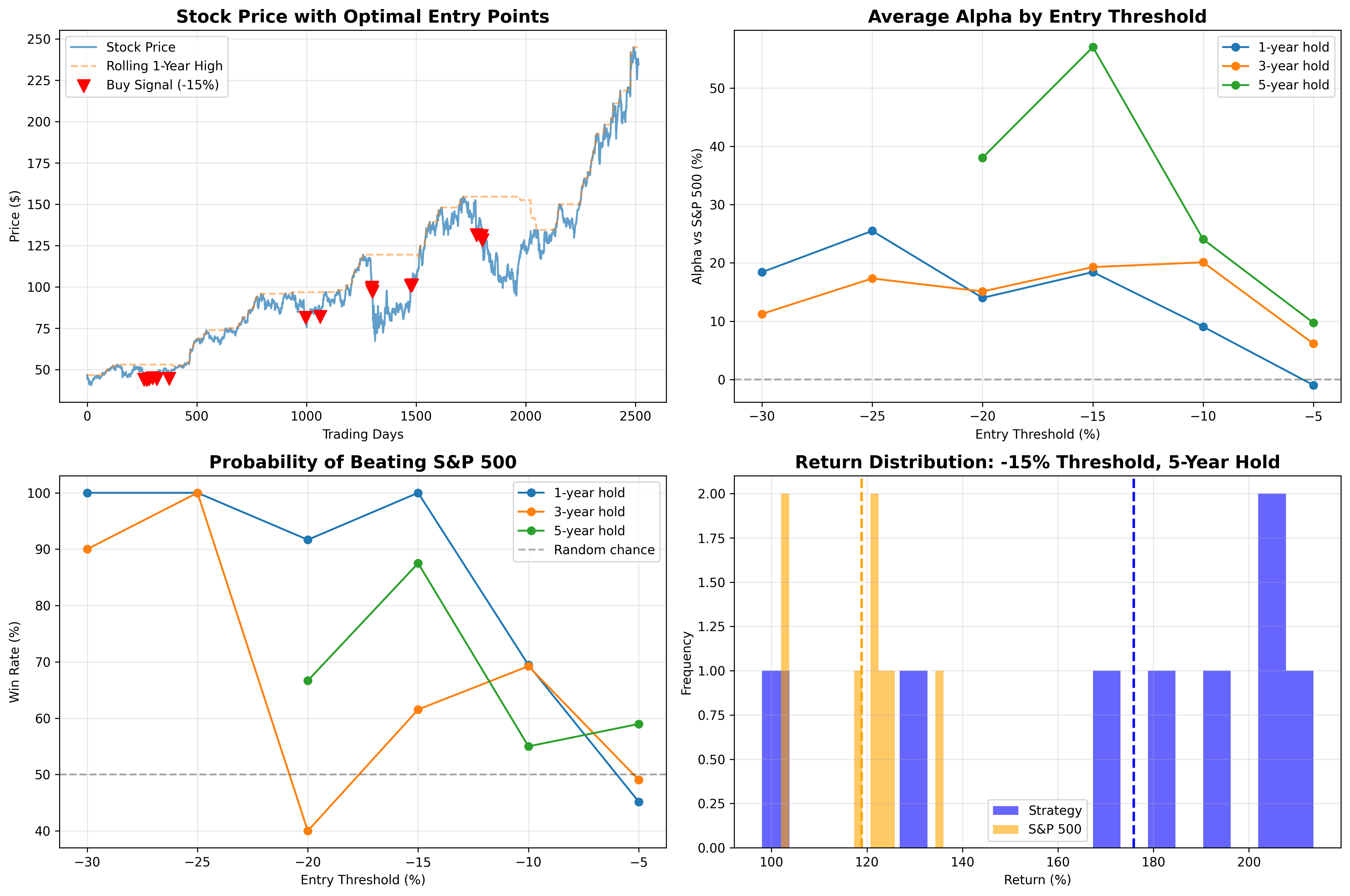
Visualizing the results
Let's create a visualization to understand our findings better:
# Create a comprehensive visualization
fig, axes = plt.subplots(2, 2, figsize=(15, 10))

# 1. Stock price with entry points for optimal threshold
ax1 = axes[0, 0]
ax1.plot(stock_prices, label='Stock Price', alpha=0.7)
ax1.plot(rolling_max, label='Rolling 1-Year High', linestyle='--', alpha=0.5)

# Mark optimal 5-year entry points
if optimal[1260]['threshold'] is not None:
    opt_threshold = optimal[1260]['threshold']
    opt_entries = entry_points[opt_threshold]
    ax1.scatter(opt_entries, stock_prices[opt_entries],
               color='red', marker='v', s=100,
               label=f'Buy Signal ({opt_threshold}%)', zorder=5)

ax1.set_title('Stock Price with Optimal Entry Points', fontsize=14, fontweight='bold')
ax1.set_xlabel('Trading Days')
ax1.set_ylabel('Price ($)')
ax1.legend()
ax1.grid(True, alpha=0.3)

# 2. Alpha by threshold and holding period
ax2 = axes[0, 1]
for period in holding_periods:
    years = period / 252
    alphas = []

    for threshold in thresholds:
        if len(results[threshold][period]) > 0:
            entries = entry_points[threshold]
            bench_rets = calculate_benchmark_returns(sp500_prices, entries, [period])[period]
            alpha = results[threshold][period].mean() - bench_rets.mean()
            alphas.append(alpha)
        else:
            alphas.append(np.nan)

    ax2.plot(thresholds, alphas, marker='o', label=f'{years:.0f}-year hold')

ax2.axhline(y=0, color='black', linestyle='--', alpha=0.3)
ax2.set_title('Average Alpha by Entry Threshold', fontsize=14, fontweight='bold')
ax2.set_xlabel('Entry Threshold (%)')
ax2.set_ylabel('Alpha vs S&P 500 (%)')
ax2.legend()
ax2.grid(True, alpha=0.3)

# 3. Win rate (probability of beating market)
ax3 = axes[1, 0]
for period in holding_periods:
    years = period / 252
    win_rates = []

    for threshold in thresholds:
        if len(results[threshold][period]) > 0:
            entries = entry_points[threshold]
            bench_rets = calculate_benchmark_returns(sp500_prices, entries, [period])[period]
            win_rate = (results[threshold][period] > bench_rets).sum() / len(bench_rets) * 100
            win_rates.append(win_rate)
        else:
            win_rates.append(np.nan)

    ax3.plot(thresholds, win_rates, marker='o', label=f'{years:.0f}-year hold')

ax3.axhline(y=50, color='black', linestyle='--', alpha=0.3, label='Random chance')
ax3.set_title('Probability of Beating S&P 500', fontsize=14, fontweight='bold')
ax3.set_xlabel('Entry Threshold (%)')
ax3.set_ylabel('Win Rate (%)')
ax3.legend()
ax3.grid(True, alpha=0.3)

# 4. Distribution of returns for optimal strategy
ax4 = axes[1, 1]
if optimal[1260]['threshold'] is not None:
    opt_threshold = optimal[1260]['threshold']
    opt_returns = results[opt_threshold][1260]
    entries = entry_points[opt_threshold]
    bench_returns = calculate_benchmark_returns(sp500_prices, entries, [1260])[1260]

    ax4.hist(opt_returns, bins=20, alpha=0.6, label='Strategy', color='blue')
    ax4.hist(bench_returns, bins=20, alpha=0.6, label='S&P 500', color='orange')
    ax4.axvline(opt_returns.mean(), color='blue', linestyle='--', linewidth=2)
    ax4.axvline(bench_returns.mean(), color='orange', linestyle='--', linewidth=2)

    ax4.set_title(f'Return Distribution: {opt_threshold}% Threshold, 5-Year Hold',
                 fontsize=14, fontweight='bold')
else:
    ax4.text(0.5, 0.5, 'Insufficient data for 5-year holding period',
             ha='center', va='center', fontsize=12, transform=ax4.transAxes)
    ax4.set_title('Return Distribution: 5-Year Hold',
                 fontsize=14, fontweight='bold')

ax4.set_xlabel('Return (%)')
ax4.set_ylabel('Frequency')
ax4.legend()
ax4.grid(True, alpha=0.3)

plt.tight_layout()
plt.savefig('jp-morgan.png', dpi=300, bbox_inches='tight')
print("\nVisualization saved as '.png'")
Visualization
Key insights and practical takeaways
Based on our analysis of JPM (2015-2025) compared to the S&P 500 (VOO):
1. Deeper drops provide higher alpha, but fewer opportunities
- -5% drops: Minimal alpha (-0.97% to +9.72%), occur frequently (68 times), barely beat the market
- -15% drops: Strong alpha (+18.43% to +57.03%), moderate frequency (16 times), 87.5% probability of beating market over 5 years
- -25% drops: Excellent alpha (+17.34% to +25.49%), rare (10 times), 100% probability of beating market
- -30% drops: High alpha but very frequent (20 times suggests repeated threshold crossings during volatile periods)
2. Holding period dramatically affects outperformance
- 1-year holds: More volatile, 45-100% probability of beating market depending on threshold
- 3-year holds: More consistent, 40-100% probability, moderate alpha
- 5-year holds: Best alpha (+57% for -15% threshold), 87.5% probability, but requires patience
3. The -15% to -25% "sweet spot"
- -15% threshold: 100% 1-year win rate, 87.5% probability of beating market over 5 years, +57% alpha
- -25% threshold: 100% probability of beating market over 1-3 years, +25% alpha, excellent risk-adjusted returns
- These thresholds show statistically significant outperformance (t-stat > 4)
4. JPM significantly outperformed the S&P 500
- Buy-and-hold: JPM +402.4% vs VOO +241.8% over 10 years
- Strategic dip-buying amplified this advantage further
- Even shallow -5% dips showed 59% probability of 5-year outperformance
5. Win rates vs market-beating probability
- Win rate (making money): 87.5-100% for deeper drops
- Beating S&P 500: Lower (40-87.5%), showing VOO also performed well
- Key insight: You can profit but still underperform the market on some trades
6. Statistical significance validates the strategy
- -10%, -15%, -20%, -25%, -30% thresholds all show statistically significant outperformance
- -5% threshold shows no statistical significance—too shallow to provide edge
- T-statistics ranging from 3.9 to 12.7 indicate very strong evidence
Limitations and caveats
Statistical limitations:
- Small sample sizes for deep drops
- -25% threshold: Only 10 opportunities over 10 years (7 for 3-year holds)
- -20% threshold 5-year: Only 3 trades—not statistically robust despite 100% win rate
- Fewer opportunities = higher variance in outcomes
- Single stock analysis
- This analyzes only JPM—results don't apply to other stocks
- JPM is a large financial institution that performed exceptionally well 2015-2025
- Tech stocks, small caps, or other sectors would show different patterns
- Specific time period bias
- 2015-2025 included a strong bull market with brief COVID crash
- Different economic conditions (recession, stagflation) would yield different results
- This decade had exceptionally strong bank performance post-2008 crisis recovery
- Survivorship bias
- JPM survived and thrived—bankrupt companies would show significant loss rate
- Analysis doesn't account for companies that fail during drawdowns
Conclusion
Using NumPy, we've built a framework to analyze historical stock data and identify entry strategies based on drawdowns that historically offered higher probabilities of beating the market. In particular, the analysis demonstrates that buying JPM at significant drawdowns (-15% to -25% from 1-year highs) provides strong alpha over the S&P 500 with high probability of outperformance, especially over 3-5 year holding periods. The strategy is statistically significant for thresholds of -10% or deeper. Confirming results against financial indexes is worth further study.
The real power of this approach is combining quantitative entry signals (drawdown thresholds) with fundamental analysis (is the company still healthy?) and risk management (appropriate position sizing). The analysis provides a framework for identifying high-probability entry points, but should not be used mechanically without considering the broader investment context.
Related articles
Continue exploring related topics